Earthquake Data Exploratory Data Analysis
Dataset Characteristics and Initial Observations
Dataset
In the above steps data were converted to the appropriate type.
All data was obtained from the USGS Common Catalog API, and was supplied in text format. Prior to this, in the Get-USGS-ComCat-Data.ipynb notebook, earthquake records for a rectangular area encompassing the continental United States were pulled using the USGS Common Catalog API. Records were restricted to those quakes occuring in 1970 or later having a magnitude greater than 2.5. API size limitations required this to be done in smaller subsets, which were partially cleaned and then then reassembled into a complete csv file. This file is the starting point for this notebook, focused on additional cleanup and EDA.
- lat, long, depth, cdi, dmin, gap, mag, mmi, rms, felt, nst, tz have been converted from string to float
- sig, tsunami have been converted to int
- magType, net, sources, status will be dummied when they are needed in later analysis
- id, code detail, ids, place, title, type, types, url are left as string values. They are informational and reference only, not needed for model learning or prediction
The dataset is incomplete for cdi, mmi, felt. This is expected, as not all information is recorded for every quake. Analysis of mmi cdi/felt relationship will be done using samples where this data exists. Likewise, dmin, gap, nst, rms, and tz have missing values. No correct or imputation is anticipated, as there ino planned analysis or modeling using these features in this project.
The Modified Mercali Intensity (mmi) is only computed for quakes that cause damage, and cdi is computed from citizen reports beginning around 2005. The full dataset will be used to examine any changes in earthquake frequency over time, and the smaller dataset of mmi/cdi will be used to calibrate the cdi intensity data. With that done, the slighty larger cdi dataset can be used to explore the relationship between magnitude and intensity, and to validate the current formulas, and to develop new, more regionally focused, formulas.
A data dictionary describing this data is availabe at https://earthquake.usgs.gov/data/comcat/data-eventterms.php
Of most importance to this project will be time, lat, long, depth, magnitude, mmi and cdi.
# Read in the dateset from csv

import numpy as np
import pandas as pd

df = pd.read_csv('./datasets/US-quake-raw.csv')
df.shape
(114503, 30)
df.info()
<class 'pandas.core.frame.DataFrame'>
RangeIndex: 114503 entries, 0 to 114502
Data columns (total 30 columns):
id         114503 non-null object
lat        114503 non-null float64
long       114503 non-null float64
depth      114498 non-null float64
alert      693 non-null object
cdi        14130 non-null float64
code       114503 non-null object
detail     114503 non-null object
dmin       68118 non-null float64
felt       14130 non-null float64
gap        105961 non-null float64
ids        114503 non-null object
mag        114503 non-null float64
magType    114417 non-null object
mmi        2955 non-null float64
net        114503 non-null object
nst        98355 non-null float64
place      114503 non-null object
rms        108641 non-null float64
sig        114503 non-null int64
sources    114503 non-null object
status     114503 non-null object
time       114503 non-null int64
title      114503 non-null object
tsunami    114503 non-null int64
type       114503 non-null object
types      114503 non-null object
tz         17198 non-null float64
updated    114503 non-null int64
url        114503 non-null object
dtypes: float64(12), int64(4), object(14)
memory usage: 26.2+ MB
# Correctly type the dataset

# convert tsunami to boolian - either a tsunami alert was issued or it wasn't
df['tsunami'] = df['tsunami'].astype(bool)

# convert times to a true datetime format
import datetime

df['time'] = df['time'].astype(int)
df['updated'] = df['updated'].astype(int)

df['time'] = df['time'].map(lambda x: datetime.datetime.fromtimestamp(int(x)/1000.0) )
df['updated'] = df['updated'].map(lambda x: datetime.datetime.fromtimestamp(int(x)/1000.0) )


# Convert alert to ordinal
#
def ordinize(strval, ordered_list, start_idx, idx_skip):
    i = 0
    for val in ordered_list:
        if strval == val:
            return i*idx_skip + start_idx
        i += 1

df['alert'] = df['alert'].apply(lambda x: ordinize(x, ['green', 'yellow', 'red'], 1, 1))
df['alert'] = df['alert'].fillna(value=0)
Missing values
- Five quakes missing depth data were deleted.
- For 86 quakes missing the type of calculation used to determine magnitude, the type was set to ‘Unknown.”
# Handle missing values

# Depth: 5 missing - delete these rows
df = df.dropna(subset=['depth'])

# magType: 86 missing,  fill with 'Unknown'  (there is one existing with Unknown)
df['magType'] = df['magType'].fillna(value='Unknown')


# cdi, mmi, felt:  Leave as NaN, analysis of mmi cdi/felt relationship will be done for existing values only
# dmin, gap, nst, rms, tz: Leave as NaN, no planned analysis or modeling uses these features, but they can be
# converted later should the need arise.

df.info()
<class 'pandas.core.frame.DataFrame'>
Int64Index: 114498 entries, 0 to 114502
Data columns (total 30 columns):
id         114498 non-null object
lat        114498 non-null float64
long       114498 non-null float64
depth      114498 non-null float64
alert      114498 non-null float64
cdi        14130 non-null float64
code       114498 non-null object
detail     114498 non-null object
dmin       68118 non-null float64
felt       14130 non-null float64
gap        105961 non-null float64
ids        114498 non-null object
mag        114498 non-null float64
magType    114498 non-null object
mmi        2955 non-null float64
net        114498 non-null object
nst        98355 non-null float64
place      114498 non-null object
rms        108641 non-null float64
sig        114498 non-null int64
sources    114498 non-null object
status     114498 non-null object
time       114498 non-null datetime64[ns]
title      114498 non-null object
tsunami    114498 non-null bool
type       114498 non-null object
types      114498 non-null object
tz         17198 non-null float64
updated    114498 non-null datetime64[ns]
url        114498 non-null object
dtypes: bool(1), datetime64[ns](2), float64(13), int64(1), object(13)
memory usage: 26.3+ MB
df.head(2)
| id | long | lat | depth | alert | cdi | code | detail | dmin | felt | ... | sources | status | time | title | tsunami | type | types | tz | updated | url | |
|---|---|---|---|---|---|---|---|---|---|---|---|---|---|---|---|---|---|---|---|---|---|
| 0 | nc1022389 | -121.8735 | 36.593 | 4.946 | 0.0 | NaN | 1022389 | https://earthquake.usgs.gov/fdsnws/event/1/que... | 0.03694 | NaN | ... | ,nc, | reviewed | 1974-12-30 13:28:16.830 | M 3.4 - Central California | False | earthquake | focal-mechanism,nearby-cities,origin,phase-data | NaN | 2016-12-14 18:02:44.940 | https://earthquake.usgs.gov/earthquakes/eventp... |
| 1 | nc1022388 | -121.4645 | 36.929 | 3.946 | 0.0 | NaN | 1022388 | https://earthquake.usgs.gov/fdsnws/event/1/que... | 0.04144 | NaN | ... | ,nc, | reviewed | 1974-12-30 09:46:54.820 | M 3.0 - Central California | False | earthquake | nearby-cities,origin,phase-data | NaN | 2016-12-14 18:02:33.974 | https://earthquake.usgs.gov/earthquakes/eventp... |
2 rows × 30 columns
Latitude and Longituded were miss-labeled on retrieval.
This is corrected here
# Oops, the latitude and longitude are swapped, need to fix the column headers to match data.

df.rename(columns={'lat': 'newlong', \
                        'long': 'newlat'}, inplace=True)
df.rename(columns={'newlong': 'long', \
                        'newlat': 'lat'}, inplace=True)
df.head(2)
| id | long | lat | depth | alert | cdi | code | detail | dmin | felt | ... | sources | status | time | title | tsunami | type | types | tz | updated | url | |
|---|---|---|---|---|---|---|---|---|---|---|---|---|---|---|---|---|---|---|---|---|---|
| 0 | nc1022389 | -121.8735 | 36.593 | 4.946 | 0.0 | NaN | 1022389 | https://earthquake.usgs.gov/fdsnws/event/1/que... | 0.03694 | NaN | ... | ,nc, | reviewed | 1974-12-30 13:28:16.830 | M 3.4 - Central California | False | earthquake | focal-mechanism,nearby-cities,origin,phase-data | NaN | 2016-12-14 18:02:44.940 | https://earthquake.usgs.gov/earthquakes/eventp... |
| 1 | nc1022388 | -121.4645 | 36.929 | 3.946 | 0.0 | NaN | 1022388 | https://earthquake.usgs.gov/fdsnws/event/1/que... | 0.04144 | NaN | ... | ,nc, | reviewed | 1974-12-30 09:46:54.820 | M 3.0 - Central California | False | earthquake | nearby-cities,origin,phase-data | NaN | 2016-12-14 18:02:33.974 | https://earthquake.usgs.gov/earthquakes/eventp... |
2 rows × 30 columns
Future plotting and display of data Discussion
Future plotting and display of data will sometimes be more convenient if the magnitudes can be grouped by decace, i.e. all earthquakes with magnitude between 3.0 and 3.999 will be grouped in decade 2.
It will also be convenient to group by year of occurance.
# Create a 'binned' magnitude column for later gropuing and plotting
# Need to make this an integer number for color coding points, so ....
# This will be called the magDecade, and will be set to the lowest integer in the decace
# Thus,  7 will mean quakes with magnitude from 7 - 7.999
#        6 will mean quakes with magnitude from 6 - 6.999   etc.


def magDecade(x):
    if x >= 8.0:
        mbin = 8
    elif x >= 7.0 and x < 8.0:
        mbin = 7
    elif x >= 6.0 and x < 7.0:
        mbin = 6
    elif x >= 5.0 and x < 6.0:
        mbin = 5
    elif x >= 4.0 and x < 5.0:
        mbin = 4
    elif x >= 3.0 and x < 4.0:
        mbin = 3
    else:
        mbin = 2   # Dataset was restricted to quakes with magnitude greater than 2.5

    return mbin

df['magDecade'] = df['mag'].apply(lambda x: magDecade(x))

df['magDecade'].value_counts(dropna=False)
2    71425
3    36662
4     5677
5      656
6       69
7        9
Name: magDecade, dtype: int64
# Create a year column for later grouping and plotting

df['year'] = df['time'].map(lambda x: getattr(x, 'year'))
df[['id','long','lat','mag','time','magDecade','year']].head(3)
| id | long | lat | mag | time | magDecade | year | |
|---|---|---|---|---|---|---|---|
| 0 | nc1022389 | -121.873500 | 36.593000 | 3.39 | 1974-12-30 13:28:16.830 | 3 | 1974 |
| 1 | nc1022388 | -121.464500 | 36.929000 | 2.99 | 1974-12-30 09:46:54.820 | 2 | 1974 |
| 2 | ci3319041 | -116.128833 | 29.907667 | 4.58 | 1974-12-30 08:12:47.870 | 4 | 1974 |
df.shape
(114498, 32)
Save the cleaned up version
# Save this cleaned up dataset for use in this and later notebooks

RUN_BLOCK = False  # Prevent execution unless specifically intended

if RUN_BLOCK:
    df.to_csv("./datasets/clean_quakes_v2.csv", index=False)
# Re-read and begin EDA
df = pd.read_csv("./datasets/clean_quakes_v2.csv")
print df.shape
df.head(3)
(114498, 32)
| id | long | lat | depth | alert | cdi | code | detail | dmin | felt | ... | time | title | tsunami | type | types | tz | updated | url | magDecade | year | |
|---|---|---|---|---|---|---|---|---|---|---|---|---|---|---|---|---|---|---|---|---|---|
| 0 | nc1022389 | -121.873500 | 36.593000 | 4.946 | 0.0 | NaN | 1022389 | https://earthquake.usgs.gov/fdsnws/event/1/que... | 0.03694 | NaN | ... | 1974-12-30 13:28:16.830 | M 3.4 - Central California | False | earthquake | focal-mechanism,nearby-cities,origin,phase-data | NaN | 2016-12-14 18:02:44.940 | https://earthquake.usgs.gov/earthquakes/eventp... | 3 | 1974 |
| 1 | nc1022388 | -121.464500 | 36.929000 | 3.946 | 0.0 | NaN | 1022388 | https://earthquake.usgs.gov/fdsnws/event/1/que... | 0.04144 | NaN | ... | 1974-12-30 09:46:54.820 | M 3.0 - Central California | False | earthquake | nearby-cities,origin,phase-data | NaN | 2016-12-14 18:02:33.974 | https://earthquake.usgs.gov/earthquakes/eventp... | 2 | 1974 |
| 2 | ci3319041 | -116.128833 | 29.907667 | 6.000 | 0.0 | NaN | 3319041 | https://earthquake.usgs.gov/fdsnws/event/1/que... | 2.73400 | NaN | ... | 1974-12-30 08:12:47.870 | M 4.6 - 206km SSE of Maneadero, B.C., MX | False | earthquake | origin,phase-data | NaN | 2016-01-28 20:48:03.640 | https://earthquake.usgs.gov/earthquakes/eventp... | 4 | 1974 |
3 rows × 32 columns
print list(df.columns)
['id', 'long', 'lat', 'depth', 'alert', 'cdi', 'code', 'detail', 'dmin', 'felt', 'gap', 'ids', 'mag', 'magType', 'mmi', 'net', 'nst', 'place', 'rms', 'sig', 'sources', 'status', 'time', 'title', 'tsunami', 'type', 'types', 'tz', 'updated', 'url', 'magDecade', 'year']
# Restrict to columns of interest
print list(df[['depth', 'alert', 'mmi', 'cdi', 'felt', 'mag', 'time']].columns)
['depth', 'alert', 'mmi', 'cdi', 'felt', 'mag', 'time']
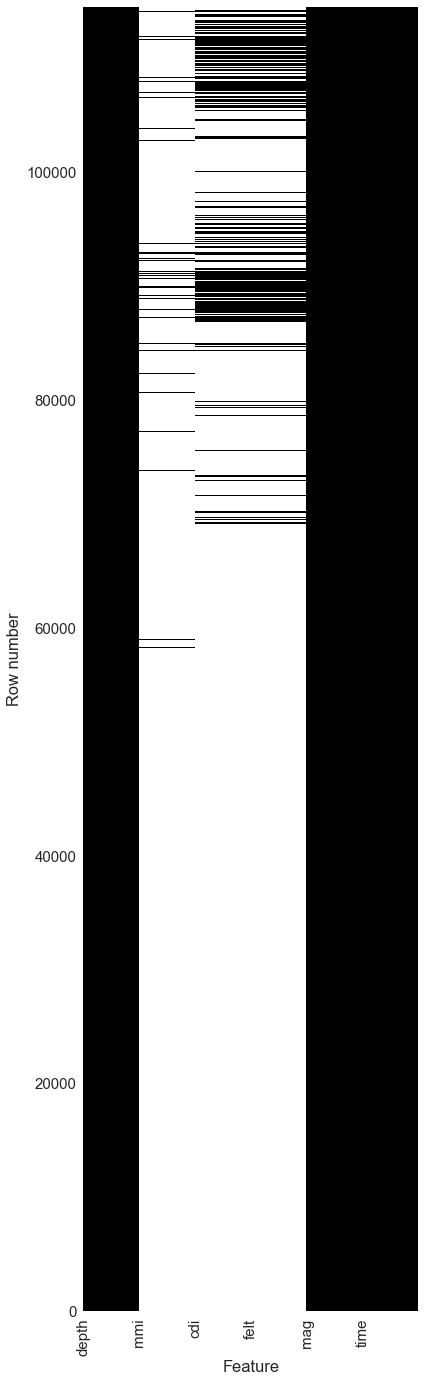
Map of missing data
Black indicates data exists, white indicates missing values
X-axis labels are on the left edge of the column they represent
This is not a surprise, as Modified Mercalli Intensity (MMI) require expert, on site visits too assess, and are generally only done for significant, damage causing quakes. CDI and Felt data comes from crowd sourced citizen reported data, and this program was only begun in the late ’90s. Also, there are few reports for low magnitude quakes that are not felt. Comparison of MMI and CDI can be done only for quakes that have values for both.
# A map of missing data.  Clearly, it will be necessary to subset the quakes to use only those that have
# available intensity data

# Seaborn set(font_scale=__) is just a quick way to adjust font scale
# for matplotlib graphs drawn after this is called
import matplotlib.pyplot as plt
import seaborn as sns
sns.set(font_scale=1.5)

fig, ax = plt.subplots(figsize=(6,24))

ax.pcolor(df[['depth', 'mmi', 'cdi', 'felt', 'mag', 'time']].isnull(), cmap='gist_gray')
ax.set_ylabel("Row number")
ax.set_xlabel("Feature")
ax.set_xticklabels(df[['depth', 'mmi', 'cdi', 'felt', 'mag', 'time']].columns, rotation=90 )
plt.show()
Reverse Geocode the latitude and longitude
I wanted to get the country, state, county, and zip code for all quakes, and use that to filter by country to get just US quakes, or to examine frequency differences by state to see if there are any regions other than Oklahoma were quake frequency is increasing.
The code below will do this, but Google limitations on the number of requests prevented this from being done for 114498 earthquaks. A future project is to determine the method and cost to process this dataset through geocode to obtain the location data.
# Create columns for geographic data

RUN_BLOCK = False  # Prevent execution unless specifically intended

if RUN_BLOCK:
    df['q_country'] = np.nan
    df['q_state'] = np.nan
    df['q_county'] = np.nan
    df['q_zip_code'] = np.nan
# Use geocode to add columns for country, state, county and postal_code

from pygeocoder import Geocoder

def is_offshore(lat, long):
    # Filter quakes off west coast before to lower the number that will be geocoded.
    if (qlat > 39) and (qlong < -124):
        return True
    elif qlong < (-114 + (qlat-26)*(-10/13.)):
        return True
    else:
        return False


RUN_BLOCK = False  # Prevent execution unless specifically intended

if RUN_BLOCK:
    quakes = []
    idxs = []
    for idx in range(114000, 114498):
        if idx % 100 == 0:
            print "Retrieving geopolitical info for records", idx, "to", idx+100
            quake_id = df.loc[idx,'id']
            quakes.append(quake_id)
            idxs.append(idx)

        if is_offshore(df.iloc[idx,2], df.iloc[idx,1]):
            country.append('offshore')
            state.append('offshore')
            county.append('offshore')
            zip_code.append('offshore')
            df.loc[idx, 'country'] = 'offshore'
            df.loc[idx, 'state'] = 'offshore'
            df.loc[idx, 'county'] = 'offshore'
            df.loc[idx, 'zip_code'] = 'offshore'

        else:
            try:
                results = Geocoder.reverse_geocode(df.iloc[idx,2], df.iloc[idx,1])
                country.append(results.country)
                state.append(results.state)
                county.append(results.county)
                zip_code.append(results.postal_code)
                df.loc[idx, 'country'] = results.country
                df.loc[idx, 'state'] = results.state
                df.loc[idx, 'county'] = results.county
                df.loc[idx, 'zip_code'] = results.postal_code

            except:
                country.append('offshore')
                state.append('offshore')
                county.append('offshore')
                zip_code.append('offshore')
                df.loc[idx, 'country'] = 'offshore'
                df.loc[idx, 'state'] = 'offshore'
                df.loc[idx, 'county'] = 'offshore'
                df.loc[idx, 'zip_code'] = 'offshore'

    print "Done retrieving reverse codes"
## Geo columns do not contain uniform data, so pickle to save dataframe as object rather than csv.

# import pickle

# pickle.dump( df, open( "clean_quakes_geocode.p", "wb" ) )

# df = pickle.load( open( "save_losers_df.p", "rb" ) )
# Check for duplicate quakes  - there seem to be none with same ID

df[df.duplicated(subset='id')]
| id | long | lat | depth | alert | cdi | code | detail | dmin | felt | ... | time | title | tsunami | type | types | tz | updated | url | magDecade | year |
|---|
0 rows × 32 columns
Exploratory Data Analysis
Now we get to the more interesting part. The cells below generate
- table of earthquake frequency by year for quakes with magnitude > 2.5 occuring in a rectangular box encompassing the continental United States.
- stacked bar charts showing frequency over time
# Earthquake Frequency

magSummary = df.groupby(['year', 'magDecade']).size().unstack()
magSummary = magSummary.fillna(0).astype(int)
magSummary.loc[1970:1984].T
| year | 1970 | 1971 | 1972 | 1973 | 1974 | 1975 | 1976 | 1977 | 1978 | 1979 | 1980 | 1981 | 1982 | 1983 | 1984 |
|---|---|---|---|---|---|---|---|---|---|---|---|---|---|---|---|
| magDecade | |||||||||||||||
| 2 | 220 | 277 | 214 | 354 | 938 | 1478 | 1123 | 869 | 936 | 1266 | 1655 | 1156 | 1467 | 2075 | 1461 |
| 3 | 175 | 474 | 171 | 227 | 677 | 967 | 615 | 491 | 528 | 786 | 1773 | 725 | 674 | 1088 | 915 |
| 4 | 11 | 57 | 14 | 68 | 138 | 163 | 126 | 72 | 112 | 108 | 537 | 98 | 104 | 149 | 127 |
| 5 | 2 | 6 | 3 | 17 | 12 | 15 | 22 | 11 | 9 | 16 | 42 | 6 | 12 | 19 | 14 |
| 6 | 0 | 2 | 0 | 0 | 1 | 2 | 2 | 0 | 1 | 1 | 6 | 1 | 0 | 2 | 5 |
| 7 | 0 | 0 | 0 | 0 | 0 | 0 | 0 | 0 | 0 | 0 | 1 | 0 | 0 | 0 | 0 |
magSummary.loc[1985:1999].T
| year | 1985 | 1986 | 1987 | 1988 | 1989 | 1990 | 1991 | 1992 | 1993 | 1994 | 1995 | 1996 | 1997 | 1998 | 1999 |
|---|---|---|---|---|---|---|---|---|---|---|---|---|---|---|---|
| magDecade | |||||||||||||||
| 2 | 1541 | 2692 | 2022 | 1532 | 1516 | 1153 | 1039 | 5418 | 1399 | 1997 | 1127 | 995 | 1252 | 1315 | 2306 |
| 3 | 680 | 1064 | 860 | 761 | 781 | 609 | 606 | 2045 | 701 | 1158 | 611 | 499 | 599 | 654 | 1196 |
| 4 | 98 | 162 | 96 | 93 | 145 | 105 | 73 | 281 | 66 | 154 | 92 | 68 | 77 | 80 | 150 |
| 5 | 5 | 20 | 9 | 15 | 9 | 16 | 10 | 31 | 9 | 18 | 7 | 13 | 12 | 6 | 10 |
| 6 | 1 | 3 | 2 | 1 | 1 | 0 | 3 | 5 | 2 | 2 | 2 | 0 | 0 | 0 | 0 |
| 7 | 0 | 0 | 0 | 0 | 0 | 0 | 1 | 2 | 0 | 1 | 0 | 0 | 0 | 0 | 1 |
magSummary.loc[2000:2016].T
| year | 2000 | 2001 | 2002 | 2003 | 2004 | 2005 | 2006 | 2007 | 2008 | 2009 | 2010 | 2011 | 2012 | 2013 | 2014 | 2015 | 2016 |
|---|---|---|---|---|---|---|---|---|---|---|---|---|---|---|---|---|---|
| magDecade | |||||||||||||||||
| 2 | 1116 | 1108 | 953 | 1122 | 1684 | 1270 | 960 | 937 | 1370 | 1109 | 3666 | 1448 | 1138 | 1324 | 2840 | 3270 | 2431 |
| 3 | 560 | 569 | 490 | 628 | 886 | 655 | 502 | 399 | 695 | 487 | 1846 | 669 | 479 | 579 | 1241 | 1428 | 1067 |
| 4 | 95 | 117 | 82 | 123 | 103 | 124 | 94 | 76 | 140 | 94 | 233 | 160 | 126 | 125 | 131 | 111 | 98 |
| 5 | 5 | 19 | 11 | 11 | 11 | 13 | 15 | 23 | 36 | 16 | 19 | 22 | 13 | 9 | 9 | 9 | 18 |
| 6 | 1 | 3 | 0 | 4 | 0 | 1 | 1 | 1 | 1 | 3 | 1 | 1 | 3 | 1 | 2 | 0 | 1 |
| 7 | 0 | 0 | 0 | 0 | 0 | 1 | 0 | 0 | 0 | 0 | 1 | 0 | 1 | 0 | 0 | 0 | 0 |
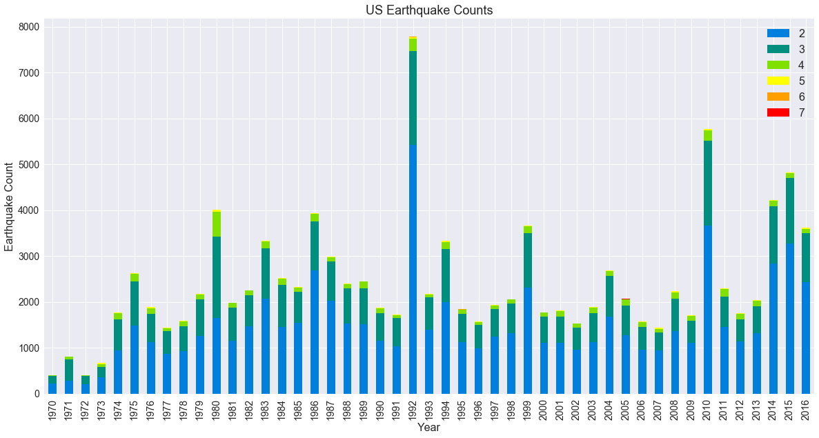
Charting Earthquake Frequency
This bar chart shows the number of earthquakes yearly, separate by magnitude. There are many more quakes of lower magnitude than higher, as we know from experience, but the year to year trends are quite variable. There were 2 large earthquakes in California in 1992, and the spike is likely to do the number of smaller aftershocks these quakes produced. The spikes in 2010 and after are influcenced by the increased number of eartquakes in Oklahoma, thought to be caused by re-injection of waste water from oil wells.
This dataset represents earthquakes entered in the USGS common catalog. These are sourced from various state and academic agencies, and the number of contributors has increased over time. The ramp up in the early 1970s is probably due to additional quakes being reported to USGS, rather than an actual sudden increase in seismic activity.
import seaborn as sns
import matplotlib.pyplot as plt

# plt.style.use('fivethirtyeight')
%matplotlib inline

q_colors = ['#007FDD', '#008E7F', '#80E100', '#FFFF00', '#FFA000', '#FF0000']
ax = magSummary.loc[1970:2016,2:7].plot(kind='bar',stacked=True, colors=q_colors, \
                                               figsize=(20, 10), legend=True, fontsize=14)


ax.set_title("US Earthquake Counts", fontsize=18 )
ax.set_xlabel("Year", fontsize=16)
ax.set_ylabel("Earthquake Count", fontsize=16)
ax.legend(fontsize=16)
plt.show()
Mapping Earthquakes
Here are two plots of earthquake locations. The circle size and color represents magnitude; larger and more toward read are higher magnitude. Notice the difference in number of quakes in Oklahoma between 2000, 2001 and 2015 to present. This is believed to be caused by re-injection of wastewater from oil wells back into the ground, where it then lubricates existing faults.
import plotly.plotly as py
import pandas as pd

import plotly
# Credentials are set at this point, but removed from blog post
df_magplot = df[(df['year'] >= 2000) & (df['year'] < 2002)]\
  [['id','mag','lat','long', 'magDecade']].sort_values('mag', axis=0, ascending=False)
df_magplot['text'] = df_magplot['id'] + '<br>Magnitude ' + (df_magplot['mag']).astype(str)
magDecades=[8, 7, 6, 5, 4, 3, 2]
colors = ["rgb(255,0,0)", "rgb(255,90,0)", "rgb(255,160,0)", "rgb(255,255,0)",\
          "rgb(128,255,0)", "rgb(0,142,128)", "rgb(0,128,255)", "rgb(0,0,255)"]
quakes = []
scale = 4
i = 0

for mbin in magDecades:
    df_sub = df_magplot[df_magplot['magDecade'] == mbin]
    quake = dict(
        type = 'scattergeo',
        locationmode = 'USA-states',
        lon = df_sub['long'],
        lat = df_sub['lat'],
        text = df_sub['text'],
        marker = dict(
            size = (df_sub['mag']**4)/scale,
            color = colors[i],
            line = dict(width=0.5, color='rgb(40,40,40)'),
            sizemode = 'area'
        ),
        name = '{0}'.format(mbin) )
    quakes.append(quake)
    i += 1

layout = dict(
        title = 'US Earthquakes 2000, 2001 to present<br>(Click legend to toggle traces)',
        showlegend = True,
        geo = dict(
            scope='usa',
            projection=dict( type='albers usa' ),
            showland = True,
            landcolor = 'rgb(217, 217, 217)',
            subunitwidth=1,
            countrywidth=1,
            subunitcolor="rgb(255, 255, 255)",
            countrycolor="rgb(255, 255, 255)"
        ),
    )

fig = dict( data=quakes, layout=layout )
py.iplot( fig, validate=False, filename='d3-bubble-map-2000-2001-magnitude' )
df_magplot = df[df['year'] >= 2015]\
  [['id','mag','lat','long', 'magDecade']].sort_values('mag', axis=0, ascending=False)
df_magplot['text'] = df_magplot['id'] + '<br>Magnitude ' + (df_magplot['mag']).astype(str)
magDecades=[8, 7, 6, 5, 4, 3, 2]
colors = ["rgb(255,0,0)", "rgb(255,90,0)", "rgb(255,160,0)", "rgb(255,255,0)",\
          "rgb(128,255,0)", "rgb(0,142,128)", "rgb(0,128,255)", "rgb(0,0,255)"]
quakes = []
scale = 4
i = 0

for mbin in magDecades:
    df_sub = df_magplot[df_magplot['magDecade'] == mbin]
    quake = dict(
        type = 'scattergeo',
        locationmode = 'USA-states',
        lon = df_sub['long'],
        lat = df_sub['lat'],
        text = df_sub['text'],
        marker = dict(
            size = (df_sub['mag']**4)/scale,
            color = colors[i],
            line = dict(width=0.5, color='rgb(40,40,40)'),
            sizemode = 'area'
        ),
        name = '{0}'.format(mbin) )
    quakes.append(quake)
    i += 1

layout = dict(
        title = 'US Earthquakes 2015 to present<br>(Click legend to toggle traces)',
        showlegend = True,
        geo = dict(
            scope='usa',
            projection=dict( type='albers usa' ),
            showland = True,
            landcolor = 'rgb(217, 217, 217)',
            subunitwidth=1,
            countrywidth=1,
            subunitcolor="rgb(255, 255, 255)",
            countrycolor="rgb(255, 255, 255)"
        ),
    )

fig = dict( data=quakes, layout=layout )
py.iplot( fig, validate=False, filename='d3-bubble-map-2015-present-magnitude' )
Earthquakes with crowd sourced Intensity data
The first modeling step of this project will be to compare the expert determined Modified Mercalli Intensity (MMI) with the Community Decimal Intensity (CDI). CDI is calculated by the USGS using “Did You Feel It” (DYFI) reports submitted on-line by those who experienced the quake and chose to contribute. This is a far more limited dataset, as Modified Mercalli Intensity (MMI) requires expert, on site visits too assess, and are generally only done for significant, damage causing quakes. CDI data collection began in the late ’90s. There are few reports for low magnitude quakes that are not felt. Comparison of MMI and CDI can be done only for quakes that have values for both. Furthermore, the quality of CDI is improved by multiple responses.
Intensity decreases with distance from the quake location, and DYFI reports reflect this. The USGS aggregates and averages reports by zip code, and provides this averaged value at latitude and longitude correpsonding to the center of the zip code region. The quality of CDI is improved by multiple responses, and so for this initial look at MMI / CDI correlation, I will use only quakes with 5 or more CDI reports, which further reduces the dataset. The maximum observed MMI and CDI for each quake will be used. This plot shows that subset of quakes, with both MMI and CDI values, with CDI computed from 5 or more DYFI reports.
df_magplot = df[(df['felt'] >= 5) & df['mmi'].notnull()]\
   [['id','mag','lat','long', 'magDecade']].sort_values('mag', axis=0, ascending=False)
df_magplot['text'] = df_magplot['id'] + '<br>Magnitude ' + (df_magplot['mag']).astype(str)
magDecades=[8, 7, 6, 5, 4, 3, 2]
colors = ["rgb(255,0,0)", "rgb(255,90,0)", "rgb(255,160,0)", "rgb(255,255,0)",\
          "rgb(128,255,0)", "rgb(0,142,128)", "rgb(0,128,255)", "rgb(0,0,255)"]
quakes = []
scale = 4
i = 0

for mbin in magDecades:

    df_sub = df_magplot[df_magplot['magDecade'] == mbin]

    quake = dict(
        type = 'scattergeo',
        locationmode = 'USA-states',
        lat = df_sub['lat'],
        lon = df_sub['long'],
        text = df_sub['text'],
        marker = dict(
            size = (df_sub['mag']**4)/scale,
            color = colors[i],
            line = dict(width=0.5, color='rgb(40,40,40)'),
            sizemode = 'area'
        ),
        name = '{0}'.format(mbin) )
    quakes.append(quake)
    i += 1

layout = dict(
        title = 'Earthquakes with MMI and CDI (from > 5 DYFI reports) data<br>(Click legend to toggle traces)',
        showlegend = True,
        geo = dict(
            scope='usa',
            projection=dict( type='albers usa' ),
            showland = True,
            landcolor = 'rgb(217, 217, 217)',
            subunitwidth=1,
            countrywidth=1,
            subunitcolor="rgb(255, 255, 255)",
            countrycolor="rgb(255, 255, 255)"
        ),
    )

fig = dict( data=quakes, layout=layout )
py.iplot( fig, validate=False, filename='d3-bubble-map-mmi-cdi-magnitude' )
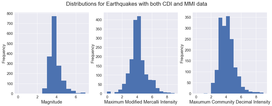
Distribution of Magnitude and Intensity data
Let’s look at the distribution of data in the final dataset, from 1970 through June of 2017, with both MMI and CDI values, and with CDI computed from 5 or more DYFI reports.
We see the dataset is limited to quakes with magnitude >= 2.5, and that MMI (expert deried) seems to assess quakes at slightly higher intensity that does CDI (crowd sourced).
dfm =  df[(df['felt'] >= 5) & df['mmi'].notnull()]
dfm.shape
(1690, 32)
sns.set(font_scale=1.5)
fig, axs = plt.subplots(ncols=3, figsize=(18,6))
fig.suptitle("Distributions for Earthquakes with both CDI and MMI data", fontsize=22)

dfm['mag'].plot(kind='hist', bins=14, range=(0,7), ax=axs[0])
dfm['mmi'].plot(kind='hist', bins=18, range=(0,9), ax=axs[1])
dfm['cdi'].plot(kind='hist', bins=18, range=(0,9), ax=axs[2])
axs[0].set_xlabel('Magnitude', fontsize=18)
axs[1].set_xlabel('Maximum Modified Mercalli Intensity', fontsize=18)
axs[2].set_xlabel('Maxumum Community Decimal Intensity', fontsize=18)
axs[0].locator_params(numticks=9)
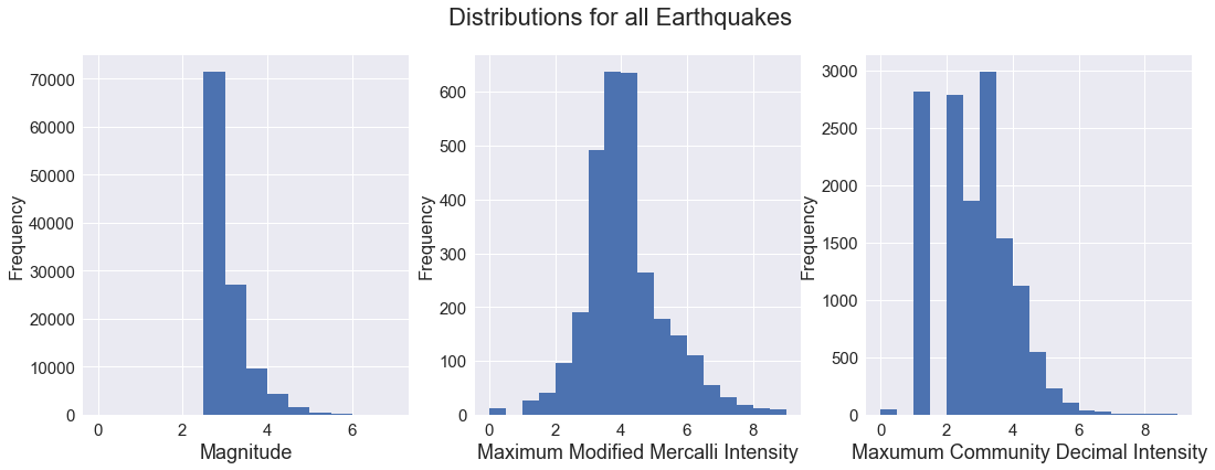
What did we lose by restricting to quakes with both MMI and CDI values, and with CDI computed from 5 or more DYFI reports? Here are similar distribution plots, but using all quakes in the dataset from 1970 onward. Observe carefuly the y-axis in these plots, as there are many quakes with neither MMI or CDI intensity measurement.
This makes is logical, remember that intensity quantifies the oberved effect of the quake, and for small quakes there may be no observed effect. MMI is never computed for these, and CDI is only reported if an individual choses to do so, and they have little motivation or interest to do so for quakes that were not felt.
While we dropped a lot of small quakes (see the magnitude distribution plot), we also dropped a lot of suspect CDI values, producing a more normally distributed dataset. There is little change in the MMI plot, because of the understandable lack of MMI assessment for small quakes.
fig, axs = plt.subplots(ncols=3, figsize=(18,6))
fig.suptitle("Distributions for all Earthquakes", fontsize=22)

df['mag'].plot(kind='hist', bins=14, range=(0,7), ax=axs[0])
df['mmi'].plot(kind='hist', bins=18, range=(0,9), ax=axs[1])
df['cdi'].plot(kind='hist', bins=18, range=(0,9), ax=axs[2])
axs[0].set_xlabel('Magnitude', fontsize=18)
axs[1].set_xlabel('Maximum Modified Mercalli Intensity', fontsize=18)
axs[2].set_xlabel('Maxumum Community Decimal Intensity', fontsize=18)
axs[0].locator_params(numticks=9)